Source release
Github repository : https://github.com/Nuand/bladeRF-adsb
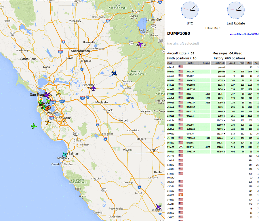
We are releasing the source to a high performance hardware accelerated ADS-B decoder that is compatible with the bladeRF. The decoder, and all relevant VHDL, C, and MATLAB design files are available. The decoder has a range of >270miles, can resolve many bit errors, and correct for packet collisions; these features that have only been available in commercial decoders until now. The decoder runs on the FPGA instead of the CPU, meaning that even a Raspberry Pi is able to handle the decoder’s maximum performance. The decoder is compatible with the dump1090 visualizer, however it simply passes fully decoded hex packets to dump1090 for displaying flights.
Pre-built bitstreams can be downloaded from https://nuand.com/fpga/
The source code and documentation are being released in conjunction with a multi-part series that explains the applied DSP theory and FPGA implementation of the ADS-B decoder.
The decoder runs on any bladeRF including the bladeRF x40 and bladeRF x115. Any low noise amplifier works with the bladeRF, however there is a bladeRF specific LNA available, the XB-300.
This multi part article will describe the design decisions and implementation of a Software Defined Radio based receiver. The article will focus on ADS-B and Mode-S.
What are ADS-B and Mode-S?
ADS-B, or Automatic Dependent Surveillance – Broadcast, is a wireless protocol used by commercial and private aircraft to identify themselves and broadcast their location in realtime. ADS-B is the digital packet format that sits on top of Mode S, the RF standard ADS-B is broadcasted over.
Why accelerate modems in hardware (with VHDL)?
Hardware acceleration allows for efficient, real-time processing of signals. An FPGA implementation of an algorithm can be designed so that a pipelined design can process a sample per clock cycle. This is not to say that a sample can be processed within one clock cycle of it arriving but rather the pipelined architecture will compute one sample per clock cycle after the pipeline fills up.
Although FPGAs have slower clock rates than processors, FPGAs can massively parallelize tasks. For applied DSP tasks, an FPGA running at 80MHz routinely outperforms an Intel i7 running at 3.5GHz. These capabilities are similar to GPGPUs. A modern GPU running CUDA or OpenCL can outperform a processor at number crunching because of the large number of parallel arithmetic cores in a GPU. So why use an FPGA for applied DSP? One main reason is cost, even the most inexpensive desktop processor setup will cost at least $150, whereas FPGAs can achieve a comparable performance for a fifth of the price. Additionally, a single chip is much smaller, more low power and power efficient than a complicated GPGPU desktop setup. Although GPGPU solutions in the same price range as FPGAs contains far more on-chip arithmetic processing power than an FPGA, FPGAs do have an added advantage. FPGAs have very a flexible programmable logic fabric that allows for clock-cycle accurate control of the FPGA’s resources. An effective engineer can utilize that level of control to do more with an FPGA running at 80MHz than a GPGPU. In my experience, GPGPUs are better suited for applications where raw computation power is needed and considerations like data latency, processing latency, and power efficiency do not matter.
What design flow is recommended?
Our preferred design flow is to model and simulate in MATLAB, implement and validate the modem using fixed-point arithmetic in C, and ultimately use the C model as a reference to implement the modem in VHDL.
MATLAB is a great tool for prototyping ideas very quickly. A few lines of Matlab can easily capture the essence of an idea that could take hours to implement in C. The goal of the ASD-B core MATLAB script is to simulate the end to end performance of the ADS-B waveform and observe how the modem reacts to expected channel effects (such as fading), and receiver phenomenon (such as DC offsets, clipping, quantization).
It is in this stage of the design that the acquisition, equalization, and decoding algorithms are developed.
Many of the channel effects, and receiver phenomenon are random number processes which means the only way to get a good understanding for the modem’s performance is to simulate many packets with similar perturbations. Some parameters such SNR, and multipath require sweeping, for example sweeping SNR from -5 dB to 3dB with 0.25dB increments is a good idea when working with a waveform that necessitates 1dB of SNR. Simulations where the SNR is swept across such a range is usually referred to as a BER (Bit Error Rate) curve and is one of the fundamental ways of characterizing the performance of a receiver.
Once the receiver architecture is validated by good simulated BER and PER (Packet Error Rate) performance, it is time to implement the modem. Going to VHDL may seem appealing at this point however it is much more time efficient to implement the modem in C. The MATLAB model uses floating point arithmetic and most of the operations are performed on vectors whereas the final VHDL implementation will be a pipelined fixed point arithmetic implementation. There are far too many design decisions that need to be made and validated in going from MATLAB to VHDL, a good intermediary step is to implement the modem in C. C provides 64bit fixed point data types and arithmetic operations, complements of the underlying x86 processor, that perfectly emulate how the VHDL implementation will work. The C implementation will work as an easy to debug implementation and good reference point for how the VHDL should behave.
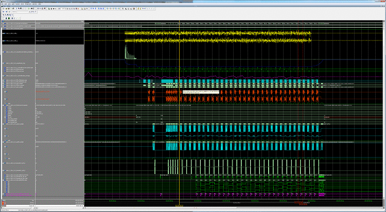
The final translation to VHDL from a fixed-point C implementation is not without challenges. The greatest challenge in implementing the modem in VHDL is, as almost always, meeting timing closure. Almost all additions can fit in one clock cycle. Some multiplications can fit in one clock system, others may not. And almost no divisions can happen in less than N/2 clock cycles (where N is the number of bits in the dividend). These simple heuristics can be used as a rule of thumb for designing the arithmetic pipelines but there will still likely be timing problems that will have to be resolved.
| Stage |
Pros |
Cons |
Notes |
|---|
|
MATLAB |
Very efficient way of prototyping algorithms
Many existing DSP and Telecomm tools |
Not real-time
Can use a lot of RAM and CPU time |
The receiver architecture and techniques should be known before progressing. |
|
C |
Can be real-time
Memory and CPU efficient
Provides bit level accurate simulations with VHDL |
Memory management |
file IO |
and all signal processing functions have to be implemented |
The sample-based fixed point implementation should be designed here. The modem should be able to match the vector-based floating point MATLAB reference modem. |
|
VHDL |
Very fast |
efficient |
and customizable |
Very hard to debug interactively
Design is no longer entirely a digital design |
some physical effects of silicon can cause the design to misbehave |
Design defensively against operations that might cause problems with timing closure |
The next article will begin diving in to the MATLAB code.
Recent Comments